Get workbook path only

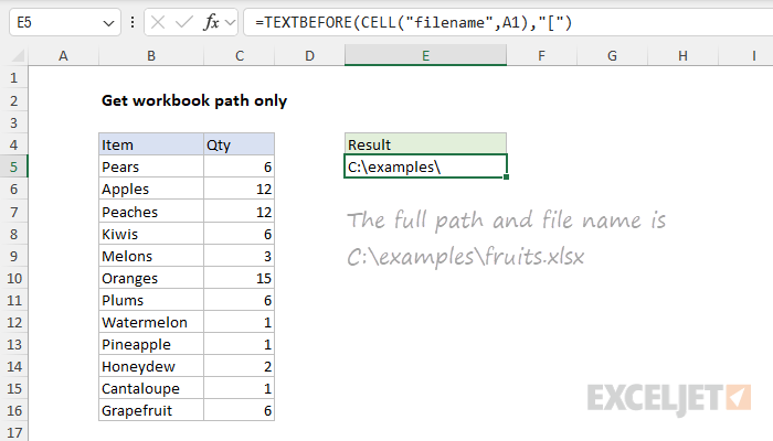
To get the path to the current workbook without the workbook name, you can use a formula based on the CELL function and the TEXTBEFORE function. In the example shown, the formula in E5 is:

=TEXTBEFORE(CELL("filename",A1),"[") 

The result is a path without the filename like this: "C:\path\".

Note: TEXTAFTER is only available in Excel 2021 and later. See below for a formula that works in earlier versions of Excel.

Generic formula

=TEXTBEFORE(CELL("filename",A1),"[")

Explanation

In this example, the goal is to get the workbook path without the workbook name. For example, given a workbook called fruits.xlsx saved to:

C:\examples\fruits.xlsx

We want the path only like this:

C:\examples\

TEXTBEFORE solution

In a modern version of Excel (Excel 2021 or later) the simplest way to solve this problem is to use the TEXTBEFORE function like this:

=TEXTBEFORE(CELL("filename",A1),"[")

TEXTBEFORE is designed to return all text before a given delimiter. Working from the inside out, the CELL function runs first and returns a full path to the workbook and worksheet:

=CELL("filename",A1) ="C:\examples\[fruits.xlsx]Sheet1"

The result is returned to the TEXTBEFORE function which is configured to return all text before the opening square bracket "[":

=TEXTBEFORE("C:\examples\[fruits.xlsx]Sheet1","[") ="C:\examples\"

The final result is the text string "C:\examples\".

Older versions of Excel

In older versions of Excel without the TEXTBEFORE function, we need to use a more complicated formula based on the LEFT function and FIND function:

=LEFT(CELL("filename",A1),FIND("[",CELL("filename",A1))-1) 

At a high level, this formula works in 3 steps:

1. Get the full path and filename with CELL
2. Locate the opening square bracket ("[")
3. Extract all text up to the opening square bracket ("[")

Get the path and filename

To get the path and file name, we use the CELL function like this:

CELL("filename",A1) // get path and filename 

The info_type argument is "filename" and reference is A1. The cell reference is arbitrary and can be any cell in the worksheet. The result is a full path like this as text:

C:\examples\[workbook.xlsx]Sheet1

Note the sheet name (Sheet1) appears at the end, and the workbook name is enclosed in square brackets, [workbook.xlsx].

Locate the opening square bracket

The location of the opening square bracket ("[") is calculated with FIND like this

FIND("]",CELL("filename",A1))-1 // returns 12 

The FIND function returns the location of "[" (13) from which 1 is subtracted to get 12. We subtract 1 because we want to remove all text starting with the "[" that precedes the workbook name. Or, to put it the other way, we want to extract all text up to the "[".

Extract path

In the previous step, we located the "]" at character 27, then stepped back to 12. This number is returned directly to the LEFT function as the num_chars argument. The text argument is again provided by the CELL function as described above:

=LEFT(CELL("filename",A1),12) =LEFT("C:\examples\[workbook.xlsx]Sheet1",12) 

The LEFT function returns the first 12 characters of text as the final result:

C:\examples\ 

The final result is the text string "C:\examples\".